- Original Article
- Open access
- Published:
Probabilistic upscaling and aggregation of wind power forecasts
Energy, Sustainability and Society volume 10, Article number: 15 (2020)
Abstract
Background
Wind power forecasts of the expected wind feed-in for the next hours or days are necessary to integrate the generated volatile wind energy into power systems. Most forecasting models predict in some sense the best value, but they ignore the other possible outcomes which may arise because of forecasting uncertainties. Probabilistic forecasts, on the other hand, also predict a distribution of possible outcomes with their respective probabilities that specific power values will occur and therefore have higher information content. In this work, we address two problems that hinder the introduction of probabilistic forecasts in practice: (1) no measurement data are available for some wind farms and (2) the flexible aggregation of probabilistic forecasts for changing wind farm portfolios.
Methods
We present an approach based on copulas that can solve both problems by modeling the spatial correlation structure between reference wind farms. By sampling from the resulting joint probability distribution, probability forecasts can be upscaled from reference wind farms to wind farms without power measurements. Furthermore, the results can be aggregated to probability forecasts of portfolios of arbitrary and changing size.
Results
We perform experiments by applying our procedure to three use cases. The results are quantitatively evaluated with different probabilistic scores. For single target wind farms, our approach is as good as a state-of-the-art reference even if no data are available for the wind farm under consideration. For portfolios, our approach also allows forecasts to be made if no data is available for some wind farms and also to aggregate flexible portfolios of changing sizes, which was not possible before.
Conclusion
Our work solves two problems that hindered the introduction of quantile probabilistic forecasts in the application. This work opens a pathway for many different applications, e.g., predictive grid securities with stochastic optimization, better marketing of renewable energies, or allow to compensate for forecast errors in various applications.
Introduction
Forecasts are an essential tool to integrate renewable energies into the energy system. The operation of the power supply system involves the complex interaction of generators, consumers, and power transmission in the power grid to balance demand and supply at each time and any location. This can only be achieved by exactly planning the operation of the equipment in detail. To this end, many tasks in the power grid require looking from minutes up to days into the future. The spatially and temporally fluctuating supply of wind energy, which is both volatile and uncertain, poses significant challenges for the power supply. The challenges are increasing with the rapid growth of this energy source. Being able to calculate these fluctuations in advance is essential for a reliable, sustainable, and economical power supply. Wind power forecasting is, therefore, necessary for integrating the ever-increasing wind energy supply into the power system. Defined more precisely, short-term wind power forecasting is the estimation of the expected power output of single wind turbines, wind farms, or a group of wind farms for the next few minutes up to several days. An overview of wind power forecasting can be found for example in the work of Monteiro et al. [1] and Foley et al. [2]. For the sake of simplicity, we do not use the term “short-term” in the following and refer to wind power forecasting only.
Probabilistic forecasts take forecast uncertainties into account and have a particular high information content. Conventional forecasts predict single values in the future for each point in time and are therefore called point forecasts or deterministic forecasts. They do not take into account that the forecast is actually subject to uncertainty and that other values besides the “best” estimate also have some probability of occurrence. Probabilistic forecasts quantify this uncertainty by predicting many values for each point in time and assigning probabilities to each of these values or predicting a continuous probability distribution. Probabilistic forecasts take possible risks into account and therefore support a secure, efficient, and cost-effective power supply. The methods can be applied in many forecast areas, e.g., the operation of the electrical grid, trading on the electricity market, the provision of control energy, and the optimal use of storages [3]. An overview of probabilistic wind power forecasting can be found in the works of Zhang et al. [4] and Bessa et al. [3]. Probabilistic wind power forecasts can be divided into physical- and statistical-based categories. Physical-based probabilistic forecasts use ensemble weather forecasts that are converted to power and calibrated to observations [5–7]. Statistical forecasts use historical weather predictions and measurements and derive intervals, quantiles, or distributions by statistical or machine learning methods [8–12]. A challenge of statistical methods that are used in this work is to model the joint distribution of several wind farms and to aggregate them correctly. Probabilistic forecasts of aggregated wind power have been studied by [13, 14]. These works assume, however, that measurements of all wind farms are available. The central assumption of the present work is that measurements are only available for individual wind farms (reference wind farms) and that the forecasts of the remaining farms must be determined by upscaling as it is often the case in practice.
Upscaling is used to supplement missing information from individual wind farms [15]. State-of-the-art forecasts require measured power data of wind farms to train the forecast models. If no data is available for some wind farms, upscaling is used for deterministic forecasts, which is a kind of extrapolation from the wind farms with available data (“reference wind farms”) to wind farms without data (“target wind farms”). In a second step, forecasts for portfolios or regions may be created by summing up the forecasts of individual wind farms (in the following called “aggregation”).
The combination of upscaling and aggregation for probabilistic forecasts was not studied before. The technique used for deterministic forecasts cannot be applied to probabilistic forecasts. In the case of deterministic forecasts, the value under consideration is only one single expectation for each time step. There exist several methods to extrapolate such scalar quantities. Also, the aggregation of deterministic forecasts is straightforward because, as required, the sum of estimated values yields the estimated value of the sum. In the probabilistic case, however, we have instead many values with assigned probabilities, which are additionally linked by their correlations. Upscaling and aggregation—or more generally the combination of probabilistic forecasts—thus have to be applied on very high dimensional joint probability distributions.
The mathematical framework to combine different probabilistic forecasts is the theory of copulas [16]. A copula is a function that separates a joint distribution of stochastic variables in the marginal distribution and the dependencies between the stochastic variables (“copula”) and thus can describe stochastic dependencies of joint distributions as the correlation between probabilistic forecasts at different locations mentioned above. The theory of copulas is used in this work to transform the forecasts into a form for which upscaling and aggregation can be applied similarly as they are applied in the deterministic case. Aggregated power forecasts based on copulas have been studied by [13, 14]. Gaussian copulas have been used, for example, by [17, 18] to model the statistical interdependence of probabilistic wind power forecasts. The problem of flexible aggregations and upscaling has not been considered yet.
With our article, we address two essential questions that frequently arise in the practical use of probabilistic forecasts:
How can aggregated probabilistic forecasts be made if not all wind farms have measurement data?
How can probabilistic forecasts be aggregated if the size of the wind farm portfolio changes?
According to the authors’ assessment, both questions have not yet been answered in the existing literature.
The article is structured as follows:
The “Method” section explains our approach, i.e., how to make probabilistic forecasts for wind farms without measurements and how to make probabilistic forecasts for portfolios based on forecasts of individual farms.
The “Verification” section introduces the evaluation measures for the probabilistic forecasts and describes the methods used to verify the results.
The “Data” section presents the data used for the experiments.
The “Experiments” section presents the set up of the experiments we use to test and evaluate the methods.
The “Results” section presents the results of the experiments as well as their evaluation and interpretation.
The “Discussion” section highlights the results and the importance of the work in current research aspects.
The “Conclusion and future work” section summarizes the work and gives an outlook on how the algorithms can be further developed.
Method
In this chapter, we describe a method to generate probabilistic forecasts of all wind farms in a portfolio. The method is based on the probabilistic forecasts of only some reference wind farms. Optionally, the method can be used to aggregate them to the total generation of the whole wind farm portfolio.
As seen in Fig. 1, we propose the following steps to create probabilistic forecasts for all wind farms in a portfolio, even if measurements of some wind farms are missing:
- 1
Create probabilistic forecasts for all reference wind farms
Fig. 1 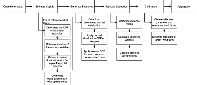
The flow diagram of the proposed method shows the main steps as well as its details
- 2
Derive the copulas from the probabilistic forecasts and the observations
- 3
Draw scenarios from these copulas
- 4
Upscale the scenarios to all target wind farm locations
- 5
Calibrate the forecasts
- 6
Optionally, aggregate the forecasts of all wind farms

For each step, different inputs are needed, and a general overview of those inputs with a short description where and why the input is needed can be found in Table 1.
Probabilistic forecasting
The uncertainty of forecasts can be described by different quantities, such as probability distributions, quantiles, or scenarios. Quantiles describe the probability of particular power levels being exceeded. Scenarios or trajectories describe possible alternative future developments and also contain information about spatial dependencies. Temporal dependencies are not crucial for our application and are therefore not considered. The scenarios created in this paper are uncorrelated in time, which does not imply any restriction for the described method. Here, we use quantiles to describe the uncertainty of individual forecasts [19] and use scenarios to describe the uncertainty and mutual correlations of forecasts for many wind farms. Scenarios are used for upscaling and aggregation; quantiles are not suitable for this because they do not contain spatial dependencies.
Quantiles are points that divide the range of probability distributions into intervals with specific probabilities. The quantile qα for nominal probability α divides the value range of the possible power values in such a way that with a probability of α the observations lie below the value of this quantile.
To predict the quantiles, the following optimization problem has to be solved for each quantile [19]:
with the observed power yt as target for all time steps t and the check function
The indicator function \(\mathbbm {1}_{x<0}\) is 1 for x<0 and 0 otherwise. The function is optimized with respect to the parameters θα. We have chosen the wind speed forecast at hub height as the predictor xt with the forecast time t. Schreiber and Sick [20] have shown that for a day-ahead forecast, wind speed is by far the most important predictor variable. All other predictors play a minor role and are therefore neglected in this study. We use quantile regression neural networks to build and train a model for Eq. (1) [21]. Figure 2 shows the resulting quantile time series qα,t together with the observed power time series yt.

The time series of a quantile probabilistic forecast. Red, observations of the power; gray, quantile intervals
Determine the copula
The quantile forecasts of the preceding section do not describe the correlations between individual sites. However, this information is crucial for upscaling and aggregation. Copulas can be used to describe the correlation structure between the wind farms [16]. More precisely, we use Gaussian copulas to estimate the covariance matrix of the forecast uncertainty between the wind farms. We choose Gaussian copulas, as they help to understand and follow each step of our method more easily. Selecting another, e.g., Student’s t or vine copula, would not change other parts of the method and have therefore not been considered here.
A similar approach was used by Pinson et al. [17] in the time frame for generating scenarios from probabilistic forecasts or by Papaefthymiou and Kurowicka [18] for spatial correlations. As soon as the Gaussian copulas and, thus, the joint distributions of all forecasts are known, we can draw samples from the joint distribution. Those samples can be upscaled to the target wind farms. From the upscaled samples, the distribution can be reconstructed.
The Gaussian copulas are determined with the four steps shown in Fig. 1. Required data are the quantiles \(q^{(i)}_{\alpha,t}\) of the probabilistic forecasts and the measured values \(y^{(i)}_{\text {ref},t}\) of all the reference wind farms \(i = 1,\dots,n\).
Determine the cumulative distribution functions
The first step is to compute an estimate \(\hat {F}^{(i)}_{t}\) of the cumulative distribution function \(F^{(i)}_{t}\) of the wind farm’s power from the quantile forecasts:
The function \(F^{(i)}_{t}\) is estimated from the m quantiles \(q^{(i)}_{\alpha,t}\) by interpolating linearly between the quantiles for each time step t and wind farm i.
Transformation to a uniform random variable
To estimate the covariance, we first have to transform the random power variable \(Y^{(i)}_{t}\) to a uniformly distributed random variable \(U^{(i)}_{t}\) with the help of the cumulative distribution function \(\hat {F}^{(i)}_{t}\) from Eq. (3):
We apply this equation to the observed power values \(Y^{(i)}_{t}\) and get new time series \(U^{(i)}_{t}\) which are uniformly distributed, as seen in Fig. 3.

The measurements and their designated quantiles they fall into. The ideal uniform distribution is marked with a dashed red line
Transformation to a normal distributed variable
Next, the uniformly distributed random variable \(U^{(i)}_{t}\) is transformed to a normal distributed variable \(V^{(i)}_{t}\)
with \(\Phi ^{-1}(x) = \sqrt {2}\, \text {erf}^{-1}(2x-1)\) and \(V^{(i)} \approx \mathcal {N}(0,1)\). The obtained normal distribution can be seen in Fig. 4.

We can see the copula created with help of the uniform distribution shown in Fig. 3. The ideal normal distribution with mean 0 and standard deviation 1 is shown as a red dashed line
Estimating the copula
Now, when all variables have been transformed into normally distributed variables, we can determine the copula to couple the forecasts of all reference wind farms. A Gaussian copula is given by the covariance matrix and is calculated by
with the forgetting factor λ∈[0,1) which sets the influence of previous estimates for Σ. Typically, with λ=0.3, good results can be achieved. If more volatile data is analyzed, a lower value of λ might be a better choice.
A further step is the normalization of the covariance to compensate for slight deviations through the update steps. This normalization step is performed by:
where ⊘ is the elementwise division and σt is the vector of standard deviations, i.e., the square root of the diagonal elements of Σt.
The copula for all wind farms can now be written as a multivariate normal distribution with covariance matrix Σt and a mean vector of μt=0.
Generate scenarios from the copula
The next step as depicted in Fig. 1 is to generate scenarios from the copula. This is done by drawing m′ samples from the multivariate normal distribution \(\mathcal {N}(\mathbf {0},\boldsymbol {\Sigma }_{t})\) estimated in Eqs. (6) and (7). We choose m′=1000. Note that the samples are correlated due to the covariance matrix. Afterward, the normally distributed variables are transformed back to variables that are distributed as the original power values by applying the same steps as for determining the copula, but in reverse order, see Eqs. (4) and (5). We continue this process for all time steps. The covariance matrix Σt is updated according to Eq. (7) as soon as new observations are available.
Next, the obtained scenarios can be upscaled to target wind farms or be aggregated to obtain the output power of a region or portfolio.
Upscaling
Upscaling is an estimated extrapolation of an overall result from a partial result. It is used if not all information for the overall result is available. In this section, we describe an upscaling algorithm for the estimation of the feedin of all wind farms from some reference wind farms, which is developed at the Fraunhofer IEE [15]. It should be emphasized that the probabilistic upscaling used in [15] adjusts quantiles to an already aggregated power and thus does not show the flexibility of the method of this paper. The upscaling algorithm uses measurements, information about the installed capacity, and location information from a few reference wind farms and determines the current feed-in of all wind farms of a specific region. The goal is to use this method for probabilistic upscaling, i.e., to find a probability distribution of all wind farms or the aggregated feed-in of a portfolio.
The power \(Y^{(i)}_{t}\) of a target wind farm at time t is determined from the power \(y^{(j)}_{\text {ref},t}\) of the reference wind farms weighted with different parameters,
where \(y^{(j)}_{\text {ref},t}\) is the measured wind energy of the jth of n reference wind farms, normalized to its installed capacity; sj,t is the status of the measurement (0 = faulty, 1 = okay), which automatically takes into account the failures or erroneous measurements; reference wind farms are indexed with j, target wind farms with i. The matrix ai,j corresponds to a distance-dependent weighting factor which is defined as
with di,j being the distance between the reference wind farm j and the target wind farm i; r is an empirically determined attenuation factor which is set here to r=50 km and can have different values for other setups. The correction factor ki,t in Eq. (8) is chosen such that the sum of the weights always is one (normalization),
This upscaling approach is applied to every single scenario generated before (see the “Generate scenarios from the copula” section). By upscaling these scenarios to the target wind farms, we extend each scenario (comprising only the set of reference farms prior to the upscaling) to a scenario comprising all wind farms (reference farms and target farms). The upscaled quantities and the extended scenarios respectively can be used in one of two ways:
The upscaled power values at a target wind farm can be used to construct a quantile forecast for this farm, comprising the quantiles \(\tilde {q}^{(i)}_{\alpha,t}\).
The extended scenarios can be used to construct a quantile forecast for all wind farms or to aggregate scenarios from a portfolio. This is done by summing up the scenarios and estimating the quantiles from the sum.
Calibration of upscaled probabilistic forecasts
If the observed frequency of measurements does not match the predicted probability, a calibration can be used to adjust the forecast based on historical measurements to the observations. Thus, it improves the reliability of a probabilistic forecast. In this section, we describe how we can calibrate the upscaled quantile forecasts and the upscaled scenario forecasts.
Calibration of quantile forecasts
Predicted quantiles \(\tilde {q}^{(i)}_{\alpha,t}\) do not necessarily correspond to the nominal probabilities α due to systematic errors in the upscaling step, i.e., \(\tilde {q}^{(i)}_{\alpha,t}\neq \hat {q}^{(i)}_{\alpha,t}\). To correct these deviations, a calibration function \(\hat {q}^{(i)}_{\alpha,t} = f_{\alpha }\left (\tilde {q}^{(i)}_{\alpha,t}\right)\) can be used which adjusts the quantiles \(\tilde {q}^{(i)}_{\alpha,t}\) [22, 23].
For the estimation of the calibration function, we use a quantile regression, similar to the probabilistic forecast in the “Probabilistic forecasting” section, but with different predictors:
where ρα is the check function defined in Eq. (2). The predictors
are composed of different upscaled quantile forecasts of the reference wind farms with a leave-one-out procedure as described below and an effective distance vector \(\boldsymbol {d}^{\text {eff}}=(d^{\text {eff}}_{1}\boldsymbol {1},\dots, d^{\text {eff}}_{n}\boldsymbol {1})\) with
The predictors \(\tilde { \boldsymbol {q}}_{\alpha }\) and deff have the same length. The parameters θα are optimized by a quantile regression. We choose a polynomial approach for the function
We have added successively further polynomial elements until no significant improvement occurs. The effective distance could be understood as follows: The further away the reference wind farms are, i.e., the larger their distance dk,l, the smaller will be their relative contribution to the calibration. Therefore, the calibration is dependent on the distance dk,l of the target wind farm k to all reference wind farms l. This distance dependence is modeled analogously to the upscaling described in the “Upscaling” section by an exponential function. Our results in the “Results of experiment 1” section suggest that the information provided by the entirety of all inter-wind farm distances can be condensed into the single quantity of the effective distance \(d^{\text {eff}}_{k}\).
We train the calibration function given by Eq. (11) using leave-one-out cross-validation: First, we additionally determine the upscaling for the reference wind farms. This is done by taking successively one wind farm l out of the set of reference wind farms {1,…,n}, and estimating its forecast by upscaling the forecasts of the remaining wind farms {1,…,n}∖{l}. As a result, the upscaled forecasts \(\tilde {\boldsymbol {q}}_{\alpha,t}\) for the reference wind farms are known in addition to the observations yt. On this data, Eq. (11) can be trained on all pairs of measurements and upscaled values simultaneously. The result is a generalized calibration model that is finally used to calibrate the quantile forecasts of the target wind farms.
Calibration of scenario forecasts
We now consider the calibration of scenario members \(\tilde {y}^{(i,k)}_{t}\) with time index t, the wind farm index i, and the member index k. The procedure must be modified in comparison to the calibration of the quantiles. First, at each point in time and for every target wind farm, the m′ scenario members have to be sorted according to their value, \(\tilde {y}^{(i,k)}_{t}\to \bar {y}^{(i,k)}_{t}\), which gives \(\bar {y}^{(i,k)}_{t}\leq \bar {y}^{(i,k')}_{t}\) for k≤k′. For each t and each i, the values \(\bar {y}^{(i,k)}_{t}\) are then interpreted as m′ quantiles with probability k/(m′+1) which can be calibrated with the steps mentioned above. After calibration, the sorting has to be reversed to obtain time-consistent scenarios again. This calibration is called ensemble copula coupling [22].
Aggregation
Often, the probabilistic forecasts of a portfolio have to be determined based on forecasts of individual wind farms. For this purpose, the individual probabilistic forecasts must be aggregated taking into account the correlations. Two cases can be distinguished here:
The aggregation of reference wind farms forecast, which corresponds to use case 2 in the “Experiments” section
The mixed aggregation of reference wind farms and target wind farms which correspond to use case 3 in the “Experiments” section
When aggregating the forecasts of the reference wind farms, scenarios with members \(y_{t}^{(i,k)}\) must first be determined according to steps 1–3 mentioned at the beginning of the “Method” section with the time index t, the wind farm index i, and the member index k. It should be noted that the copula makes the samples of the wind farms stochastically dependent on each other. Per member index and time, the scenarios then simply have to be summed up over the wind farms \(y_{t}^{(\text {agg},k)}=\sum _{i} y_{t}^{(i,k)}\). If necessary, quantiles can be determined from these scenarios.
If forecasts of reference wind farms and target wind farms have to be aggregated, then the aggregation consists of two sums:
The first sum is the sum over the scenarios of the reference wind farms I, and the second sum is the sum over the calibrated scenarios of the target wind farms J (I∩J=∅). The scenarios of the target wind farms have been estimated by upscaling the scenarios from the reference wind farms and their calibration, i.e., steps 4 and 5 mentioned at the beginning of the “Method” section. If necessary, quantiles can be determined from these scenarios.
Verification
Verification is the process of determining the quality of a prediction or upscaling. It is the comparison of an estimated quantity with an observation. The evaluation of probabilistic predictions differs significantly from point predictions since different attributes must be considered for a comprehensive evaluation, see Murphy and Epstein [24] as well as Jolliffe and Stephenson [25]. Essentially, in addition to the proximity of the forecast to the observations, the shape of the distribution must also coincide with the forecast uncertainties. The related attributes are the resolution, i.e., the width of the forecast interval or spread, respectively, as well as reliability [26]. To evaluate our results, we use the continuous ranked probability score and the reliability diagram, which are described in the following.
Continuous ranked probability score
We use the continuous ranked probability score (CRPS) to verify our forecasts [27]:
F(y) is the cumulative probability of our quantile forecast, and Fobs(y) the cumulative probability of the observation, i.e., a step function from 0 to 1 at the observation. The smaller the CRPS, the better are the results. For deterministic forecasts, this equation simplifies to the mean absolute error.
The continuous ranked probability skill score (CRPSS) can be defined from the CRPS
The normalization CRPSclim is the CRPS of the climatology, i.e., of the distribution of the observations over the total time period under consideration. The value CRPSS=1 corresponds to a perfect forecast, whereas CRPSS=0 characterizes a forecast that performs equal to climatology.
For the evaluation of the results, we also use a paired difference test, which we want to describe in the following paragraph. It is often the case that a model a is used to calculate forecasts for several locations i and that these are to be compared to the results of another model b at the same location. The model a gives the scores \(\text {CRPSS}^{a}_{i}\), and the model b the scores \(\text {CRPSS}^{b}_{i}\). If the distributions of these scores are calculated separately and then compared, it is difficult to estimate the significance of the difference. It is better to calculate the paired difference score by calculating the distribution of the paired differences of \(\text {CRPSS}^{a}_{i}-\text {CRPSS}^{b}_{i}\). We use this paired difference CRPSS to evaluate the results of experiment 1 in the “Results” section.
Reliability diagram
We also use one of the attributes of the accurate probability forecast to verify our forecast reliability. Reliability is the agreement between forecast probability and the mean observed frequency. We represent it as a reliability curve or reliability diagram, see Fig. 5 for a schematic representation. The reliability diagram draws the observed frequency against the forecast probability and shows how well the predicted probabilities are aligned with the corresponding observed frequencies. To draw a conclusion regarding the agreement between predicted and observed probability, we compare the reliability curve with a straight diagonal line, which results from the case of a perfectly reliable forecast. If the reliability curve lies below this diagonal line, there is under-forecasting. If the curve lies above the diagonal line, there is over-forecasting. For perfectly calibrated predictions, the reliability curve should be as close as possible to the diagonal line.

Schematic reliability diagram. Blue: the observed relative frequency is plotted against the forecast probability. The black straight line corresponds to a perfect reliable forecast
To build the reliability curve from the time series of power measurements y=(yt=1,…,yt=T) and a quantile time series forecast \(\hat {\boldsymbol {q}}_{\alpha } = (\hat {q}_{\alpha,t=1},\dots,\hat {q}_{\alpha,t=T})\) with probabilities α∈{α1,…,αm},αi∈[0,1], we proceed in the following way:
For each probability α∈{α1,…,αm}, the amount Obsi of power measurements that is equal to or less than the corresponding quantile forecast at that time is determined, i. e.,
$$\text{Obs}_{i} = \sum_{t} \mathbbm{1}(y_{t} \leq \hat{q}_{\alpha,t}). $$The observed conditional frequency fObs,i corresponding to probability αi is computed by dividing that number by the total amount of observations, i. e.,
$$f_{\text{Obs},i} = \frac{\text{Obs}_{i} }{T}. $$The blue curve in the reliability diagram shown in Fig. 5 is obtained by plotting all observed conditional frequencies fObs=(fObs,1,…,fObs,m) against (forecast) probabilities α=(α1,…,αm).
Data
In this study, 20 wind farms located in the northern part of Germany where used, see Fig. 6. The study is based on two data sets. The first data set contains the (current) production, and the second data set contains the probabilistic day-ahead forecasts of the wind farms’ production. We use a time series with a time range over the two complete years 2008 and 2009. The data from the year 2008 is used to train the models; the data from the year 2009 is used to verify the results. The temporal resolution of the data set is 1 h.

The locations of the 20 wind farms used in the experiments (blue circles)
Generation data
The ForWind - Center for Wind Energy Research provided the time series of the wind farm’s generation. It is a simulated data set based on the COSMO-EU analysis from the Germany Weather Service and the MERRA re-analysis data from NASA [28].
COSMO-EU is the regional numerical weather forecast model of the German Weather Service for the area Europe. The data set contains various meteorological parameters in hourly resolution with a spatial resolution of 7 km horizontally (vertical 40 grid layers from the ground up to 24 km height).
MERRA is the abbreviation for Modern-ERa Retrospective Analysis for Research and Applications. It is a NASA re-analysis for the satellite ERA using the Goddard Earth Observing System Data Assimilation System Version 5 (GEOS-5). The project focuses on the historical analysis (1979–today) of the hydrological cycle within the atmosphere.
The MERRA data covers a more extended time range whereas the COSMO-EU has a higher spatial resolution. Therefore, the COSMO-EU data was used to downscale the MERRA data to a higher resolution to yield a long time range. In this work, we use the same data as in the work of Baier et al. [15], in which different upscaling methods were compared. Thus, the studies can be easily compared. Furthermore, the data set is very large, so that the number of wind farms can be easily scaled. The following steps were performed to generate the power time series from the two basic data sets (it should be noted that the notation in this chapter is self-contained but partly overlaps with the rest of the paper):
- 1.
Bilinear remapping. Wind velocity fields of the MERRA re-analyses are bilinearly interpolated to the higher resolution COSMO-EU grid.
- 2.
Vertical extrapolation. Velocity fields are extrapolated to an altitude h (140 m) using the logarithmic wind profile
$$ w^{\text{remap}}(x,y,z=h,t)=w_{0}^{\text{remap}}(x,y,t)\frac{\ln(h/z_{0}(x,y))}{\ln(h_{0}/z_{0}(x,y))} $$(17)with the wind speed w0 at reference height h0 (50 m) and the roughness length on the ground z0.
- 3.
Bias correction. The reduced wind speed w′ results from
$$ w'(x,y,t) = \sigma_{a}(x,y,z=h)w^{\text{remap}}(x,y,z=h,t) $$(18)with the BIAS σ and
$$ \ln(\sigma_{a}(x,y,z))=\left\langle\ln\left(\frac{w_{\text{ref}}(x,y,z,t)}{w(x,y,z,t)}\right)\right\rangle $$(19)Here a, stands for the base year (a=2012) and 〈·〉 is an average. The parenthesis 〈·〉 stands for the arithmetic mean over all time steps in the base year a. wref is the reference wind speed field which originates from the COSMO-EU analyses.
- 4.
Modeling the wind energy production. The conversion of the wind speed into a wind energy production is done via
$$ P(x,y,t)=P^{\text{nom}}(x,y)\Phi(w'(x,y,t)) $$(20)with the equivalent power curve Φ published by McLean [29]. Pnom(x,y) is the installed power at the location (x,y).
Forecast data
The wind power forecasts are based on weather forecasts of the weather model COSMO-EU [30, 31]. We use the forecast run at 0:00 o’clock UTC and forecast horizons from 24 to 48 h for the following day in one-hourly temporal resolution. This data is used as input data for our forecast model which is trained to predict a relationship between wind speed and observed power to produce probabilistic day-ahead forecasts for all wind farms as described in the “Probabilistic forecasting” section. We use 20 equidistant quantiles and add two lower and two upper quantiles to resolve the tails of the distribution:
A total of 24 quantiles are therefore forecasted. These 24 quantiles are inputs to the probabilistic upscaling procedure.
Experiments
We conduct three different experiments, which correspond to typical real-world use cases, to test the performance of our method. The use cases are as follows: UC 1: Probabilistic upscaling. Probabilistic forecasts are done for all reference wind farms. The forecasts of the target wind farms are done by upscaling from these reference wind farms. This use case is relevant, if the probabilistic forecast for a single wind farm is required, even though no measurement data for this wind farm exist. UC 2: Probabilistic aggregation. All wind farms are reference wind farms for which a probabilistic forecast can be made directly. The goal is to determine the probabilistic forecast of the total feed-in. UC 3: Probabilistic upscaling and probabilistic aggregation. Not all wind farms are reference wind farms. In a first step, the probabilistic forecasts of the non-reference farms are estimated by upscaling the forecasts from the known reference wind farms to these target wind farms, followed by a probabilistic aggregation. This use case is a mixture of use cases 1 and 2.
In the following, the three experiments which belong to the use cases are described. All experiments are based on 20 wind farms for which measurements are available. The wind farms are located in the northern part of Germany, see Fig. 6 for their locations. Depending on the experiment, a subset of the wind farms is used as reference wind farms for which the power measurements were explicitly used, whereas the remaining wind farms are target wind farms and their power measurements were only used for validation.
For the reference wind farms, the following information is used:
Location name
Location coordinates
Installed power
Production data (given as synthetic time series with a resolution of 1 h)
Quantile forecasts
For the target wind farms, only the following information is used:
Location name
Location coordinates
Installed power
The experimental setup and execution of the experiments are as follows: Exp. 1: Probabilistic upscaling from reference wind farms to one single target wind farm (use case 1). The task is to forecast single wind farms based on reference wind farms. The experiment covers 20 different setups which are constructed as follows: 10 setups are created by selecting 5 fixed reference wind farms and iterating the target wind farm and 10 more setups are created by selecting one fixed target wind farm and iterating the 5 reference wind farms. All setups are shown in Fig. 7. Exp. 2: Probabilistic aggregation of the forecast for reference wind farms (use case 2). That is, it is assumed that the data of all wind farms is available and no upscaling is needed. The task is to determine a probabilistic forecast for the total production based on individual forecasts. Exp. 3: This experiment is a combination of the two experiments mentioned above (use case 3). In this experiment, a mixture of reference wind farms and wind farms without measurements are used. The task is to estimate a probabilistic forecast for the total production of all wind farms based on the forecasts from the reference wind farms. The setup is shown in Fig. 8.

Setup of exp. 1: reference wind farms (blue circles) and target farm (red circle). For the first 10 setups, the reference wind farms are fixed, and for the last 10 setups, the target wind farm is fixed. The gray circles describe the unused wind farms

Setup of exp. 3: reference wind farms with measurement data (blue circles) and wind farms without measurement data (red circles). Within this experiment, the total aggregated production of all twenty farms (with and without measurements) is considered
We apply the method from the “Method” section to these experimental setups. Then, we verify the forecast results by comparing them to the observation.
Results
In the following, we present the results of the experiments described in the “Experiments” section, in which the proposed methods of the “Method” section for probabilistic upscaling and aggregation were applied. The scores defined in the “Verification” section are used to verify and quantify the results. The results are presented in the order of the experiments.
Results of experiment 1
Figure 9 shows the quantile time series of a single wind farm for the following:
The upscaled forecast without calibration
Fig. 9 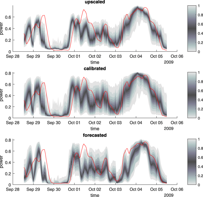
Quantile time series for one single wind farm (gray) and observations (red) for exp. 1. From top to bottom: upscaled quantile forecasts from reference wind farms, calibrated quantile forecasts, and reference quantile forecasts trained on observations. For this plot, a week with maximal fluctuations has been selected
The upscaled forecast with calibration
The hypothetic result of the forecast if data for this wind farm would be availableFootnote 1

The observations are shown for comparison. Some special characteristics are noticeable: The upscaled forecast has a systematic deviation from the observations. This is an indication that the upscaling is less reliable than the reference. The calibration significantly widens the distribution, removes the bias, and improves the reliability. The higher spread of the distribution is plausible since observations are not available for target wind farms and this is reflected in a larger uncertainty of the forecast. It should be noticed that these deviations are particularly pronounced as relatively few reference wind farms have been used. In a real-world application, more reference wind farms would have been selected, leading to more precise results than depicted here.
With the reliability plots in Fig. 10, we compare the forecasted distributions of those three forecasts to the distribution of the observations. The diagonal would indicate exact accordance with observations, i.e., perfect reliability. Upscaled forecasts without calibration deviate significantly from the expected result. Calibration brings the distributions much closer to the correct distribution. Quantile forecasts for the hypothetic case that observations for the target wind farms are available are only slightly better. These results are quantified by the CRPSS in Fig. 11. The CRPSS is calculated from Eq. (16) for all wind farms separately and shown as box plotsFootnote 2, see Fig. 11 on the left for the three cases calibrated forecasts, uncalibrated “raw” forecast, and reference forecast for which observations are available.

Reliability plots of single wind farms in exp. 1 for the three cases: (a) the upscaling without calibration (blue colored circles), (b) the upscaling with calibration (red colored squares), and (c) the hypothetic result of the forecast if data was available for this wind farm (yellow-colored diamonds)

Left: the box plot of the CRPSS of exp. 1 for a single wind farm for (a) the upscaling without calibration (“raw”), (b) upscaling with calibration (‘’calibrated”), and (c) for the hypothetic result of the forecast if observations were available for this wind farm (“reference”). Larger CRPSS values are better. Right: box plot of the paired difference CRPSS. (a) The paired difference CRPSS of the calibrated versus the uncalibrated forecast. (b) The paired difference CRPSS of the calibrated versus the reference forecast
Upscaling without calibration is often worse than the reference. Calibration improves the results significantly, but the bars overlap such that the significance of the results is not clearly visible. Therefore, the paired difference CRPSS is shown in Fig. 11a box plot of the location-wise difference between the CRPSS of the calibrated (“calibrated”) and the uncalibrated (“raw”) forecasts, i.e., \(\text {BoxPlot}(\text {CRPSS}^{\text {cal}}_{i}-\text {CRPSS}^{\text {raw}}_{i})\) instead of \(\text {BoxPlot}(\text {CRPSS}^{\text {cal}}_{i})\) and \(\text {BoxPlot}(\text {CRPSS}^{\text {raw}}_{i})\) as in the left figure. It can be seen that calibration leads to a significant improvement in all but few cases. In addition, also, the paired difference CRPSS is shown in Fig. 11b the box plot of the difference between the CRPSS of the calibrated and the reference forecast (“reference”), i. e., \(\text {BoxPlot}(\text {CRPSS}^{\text {cal}}_{i}-\text {CRPSS}^{\text {ref}}_{i})\). For most cases, the calibrated forecast is better than the reference with few outliers.
In this experiment, we have examined the performance of the approach if based on probabilistic forecasts of reference wind farms the probabilistic forecasts of target wind farms are estimated based on probabilistic upscaling. We have compared the results to reference forecasts. If the results are calibrated, our upscaling approach is better than the reference in most cases with only a few outliers.
Results of experiment 2
An excerpt from the quantile time series of the total aggregated wind farm’s power together with the aggregated power observations from all wind farms is shown in Fig. 12. The chosen time range matches the one used within the exemplary quantile time series plot of the results of Exp. 1 that is shown in Fig. 9. The forecast seems quite reasonable and, in general, captures the aggregated observations quite well. At some times, however, the outer quantiles do not seem to be broad enough to capture the observed power spectrum. This fact is also reflected in the reliability plot given in the left part of Fig. 13, which shows that the lower quantiles tend to be too high and that the higher quantiles tend to be too low.

Result of the probabilistic aggregation (exp. 2): quantile time series plot of the aggregated power of all reference wind farms (gray) and the aggregated observations of these wind farms (red)

Reliability plots for the quantiles of the power sum resulting from the aggregation over all wind farms obtained within exp. 2 (left side) and exp. 3 (right side)
The CRPSS associated with our probabilistic forecast is 0.547, which lies slightly above the average performance between a perfect forecast and the climatology. Since this experiment involves neither upscaling nor calibration, the observed deviations of the probabilistic forecast from the aggregated observations are solely due to errors of the underlying reference forecasts and due to the copula. This is, for example, reflected in the lower part of Fig. 9, which shows that on October 3, the reference forecast is not able to adequately capture the power increase observed for this specific wind farm on that day. The same is also true for the aggregated forecast shown in Fig. 12 which on October 3 is not steep enough compared to the aggregated observed power.
In this experiment, we have studied the performance of our forecasting approach if the sum of the power of all wind farms is estimated solely based on the individual probabilistic forecasts of the involved single wind farms (i.e., every wind farm is considered a reference wind farm) by means of probabilistic aggregation. We found that the approach works quite well and that the observed errors are most likely due to the errors of the underlying reference forecasts.
Results of experiment 3
Figure 14 shows excerpts from the quantile time series of the aggregated power of all wind farms (whereby the aggregation runs over all wind farms, i.e., over farms with and without measurement data) together with the aggregated power observations from these wind farms. The results shown in the upper part of the figure were obtained by leaving out the calibration step of the upscaled scenarios of wind farms without measurements, as it was described at the end of the “Calibration of upscaled probabilistic forecasts” section. The results shown in the lower part of the figure are based on additionally carrying out this scenario-calibration step as opposed to the results shown in the upper part. By comparing the two quantile forecasts shown in Fig. 14, the influence of calibrating the upscaled scenarios can be studied independently from the rest of the presented forecasting framework (upscaling and aggregation).

Result of the probabilistic upscaling and probabilistic aggregation (exp. 3): quantile time series plot of the aggregated power of all reference wind farms and target wind farms (gray) and the aggregated observations of these wind farms (red). Upper plot: aggregated power forecast obtained without calibrating the upscaled scenarios of the wind farms without measurements. Lower plot: aggregated power forecast obtained with calibrating the upscaled scenarios of the wind farms without measurements (as described at the end of the “Calibration of upscaled probabilistic forecasts” section)
First of all, we observe that the probabilistic forecast obtained without calibration resembles the one that we obtained in exp. 2 (see Fig. 12) and thereby shares its characteristics regarding the systematic deviation from the aggregated observations and the fact that some points in time the forecast’s range is not broad enough to capture the observed power spectrum, which is again reflected in the reliability plot given in the right part of Fig. 13 (blue circles). The value of the CRPSS of the probabilistic forecast without calibration is 0.549 which affirms an overall forecasting performance that is very similar to the results obtained in exp. 2. Since the only difference between these two results is the implementation of the upscaling step for the wind farms without measurements in exp. 3, we come to the conclusion that this upscaling works very well and that the observed forecasting errors are primarily due to errors of the underlying reference forecasts.
Taking into account the results obtained by additionally applying the calibration step, we see that the calibration widens the margins of the power forecast distribution in a slight but highly reasonable way, see the right part of Fig. 13 (orange squares). Although the lower quantiles of the calibrated aggregated power forecast still seem to be a bit too high and the forecast slightly tends to overestimate the aggregated power, the observed bias shift resulting from the calibration improves the forecasting performance and results in a CRPSS of 0.561.
In this experiment, we have studied the performance of our forecasting approach if the sum of the power of all wind farms (some with measurement data and some without) is estimated based on the individual probabilistic forecasts of the involved single wind farms with measurement data (the reference wind farms) by means of probabilistic upscaling, calibration (optional), and aggregation. In case the calibration step is skipped, the observed forecasting performance was very similar to the one obtained in exp. 2. Calibrating the upscaled scenarios results in the best performance compared to the results of exp. 2 and exp. 3 without calibration. The CRPSS value that results from calibration of the upscaled scenarios lies even above the value obtained in exp. 2. This shows the significance of the calibration step, which improves the forecast’s reliability and potentially fixes errors in the correlations that have not been modeled adequately before.
We note that the presented approach provides a fundamentally well-functioning way of probabilistic upscaling and aggregation of wind farm power forecasts.
Discussion
The result of the present work is a model of the joint probability \(p\left (\hat {y}^{(1)}_{t},\dots,\hat {y}^{(n)}_{t}\right)\) of the forecasts of n wind farms, where \(\hat {y}^{(i)}_{t}\) is the forecasted power of the nth wind farm. It is noteworthy that also forecasts of wind farms are taken into account, for which no power measurements are available. For this purpose, an upscaling algorithm is used, which is described by Baier et al. [15] and transferred here to a probabilistic case. This procedure differs from the work of Papaefthymiou and Kurowicka [18], in which the joint probability is formed, but measurements of all wind farms must be available. From the model of this work, probabilistic forecasts of arbitrarily aggregated portfolios can be generated. In other studies, probabilistic forecasts of aggregated power values are also considered, but models are constructed that are only optimized for a specific aggregation and are therefore inflexible [13, 14]. The joint probabilities in this paper are constructed based on statistical probabilistic forecasts. The use of ensembles of weather forecasts is not considered here. Like all statistical approaches, the distributions are optimized on historical data and cannot predict exceptional weather events, which can be forecasted only physically. An essential part of the described method is the calibration step, which especially considers the upscaling step and significantly improves the results. This calibration is also independent of a previously defined portfolio. The present work extends the existing work on probabilistic forecasts and supplements two aspects in particular: unobserved wind farms and the aggregation of forecasts of flexible portfolios. This novelty is especially crucial in practice.
Conclusion and future work
In this work, we have presented a novel approach to upscale and aggregate statistical-based probabilistic forecasts for wind farms based on a combination of copula theory and an upscaling method. The results have been applied to three different use cases:
- 1.
Estimating the probabilistic forecast of individual target wind farms by upscaling from the probabilistic forecast of reference wind farms
- 2.
Estimating the probabilistic forecast for a portfolio of reference wind farms
- 3.
A combination of use cases 1 and 2—the estimation of the probabilistic forecast of a portfolio of wind farms consisting of reference wind farms and target wind farms
We have used the data of 20 different wind farms scattered around northern Germany for these experiments. The results of the experiments are promising and show the applicability of our approach. With our approach, the power production of individual portfolios or regions can be aggregated based on only a few reference wind farms, while no measurement data of the feed-in of the portfolio’s remaining non-reference wind farms is required. The aggregation step of our method allows for a flexible creation of any required portfolio. Furthermore, the portfolio can be modified at anytime without having to create the forecast model from scratch again.
The aggregation step allows our method to create a portfolio as required and to change it at anytime without having to create the forecast model from scratch again. Since a similar procedure has not yet been published, there is no reference to which the quality of our approach can be compared. We have thus presented a method that can be used as a reference to develop the performance of this type of forecast further.
We note that the presented statistical probabilistic forecast is not about surpassing ensemble-based physical methods. The strength of ensembles lies in its ability to accurately predict future weather risks, while statistical methods tend to aim for good reliability.
The presented results will be followed by further work, e.g., the methods can be applied and verified using real data and more reference wind farms. The method can be applied to short-term forecasts with a forecast horizon of less than a few hours.
Our sampling does not depend explicitly on time. The explicit consideration of time dependencies can be taken into account if the correlation matrix is also extended to the temporal dimension, as described in Pinson et al. [17].
Many applications are possible, e.g., predictive grid security with stochastic optimization, marketing of renewable energies, dimensioning of control power to compensate for forecast errors, optimal operation of electricity storage facilities, and many more. The method presented closes an important gap in the application of probabilistic forecasts and thus opens up a broader field of potential applications.
Notation
q: Quantile forecast; \(\tilde {q}\): Upscaled quantile forecast; \(\hat {q}\): Upscaled and calibrated quantile forecast; x: Predictor (e.g., wind speed); y: Measured power; ys: Power of a portfolio; α: Nominal probability; □t: Variable at time t; T: Number of time steps; \(\Box _{t}^{(i)}\): ith wind farm at time t; \(\Box _{t}^{(i,k)}\): kth member for wind farm i at time t; n: Number of reference wind farms; m: Number of quantiles; m′: Number of scenarios; \(\hat {F}\): Estimated cumulative distribution function; Σ: Covariance matrix; r: Radius of influence; dij: Distance between wind farm i and j.
Notes
Only wind farm number 8 is shown.
In a box plot, the central line marks the median, the bottom and top edges of the box indicate the 25th and 75th percentiles, and the whiskers extend to the most extreme data points. The red crosses are outliers.
Abbreviations
- COSMO-EU:
-
Consortium for Small-Scale Modelling Europe
- CRPS:
-
Continuous ranked probability score
- CRPSS:
-
Continuous ranked probability skill score
- Exp.:
-
Experiment
- GEOS-5:
-
Goddard Earth Observing System Data Assimilation System Version 5
- MERRA:
-
Modern-ERa Retrospective Analysis for Research and Applications
- UC:
-
Use case
References
Monteiro C, Bessa R, Miranda V, Botterud A, Wang J, Conzelmann G (2009) Wind power forecasting: state-of-the-art 2009. Argonne National Laboratory (ANL), Argonne.
Foley AM, Leahy PG, Marvuglia A, McKeogh EJ (2012) Current methods and advances in forecasting of wind power generation. Renew Energy 37(1):1–8.
Bessa RJ, Möhrlen C, Fundel V, Siefert M, Browell J, Haglund El Gaidi S, Hodge B-M, Cali U, Kariniotakis G (2017) Towards improved understanding of the applicability of uncertainty forecasts in the electric power industry. Energies 10(9):1402.
Zhang Y, Wang J, Wang X (2014) Review on probabilistic forecasting of wind power generation. Renew Sust Energ Rev 32:255–70.
Ren Y, Suganthan P, Srikanth N (2015) Ensemble methods for wind and solar power forecasting—a state-of-the-art review. Renew Sust Energ Rev 50:82–91.
Taylor JW, McSharry PE, Buizza R (2009) Wind power density forecasting using ensemble predictions and time series models. IEEE Trans Energy Convers 24(3):775–82.
Pinson P, Nielsen HA, Madsen H, Kariniotakis G (2009) Skill forecasting from ensemble predictions of wind power. Appl Energy 86(7-8):1326–1334.
Bremnes JB (2004) Probabilistic wind power forecasts using local quantile regression. Wind Energy Int J Prog Appl Wind Power Convers Technol 7(1):47–54.
Wang J, Botterud A, Bessa R, Keko H, Carvalho L, Issicaba D, Sumaili J, Miranda V (2011) Wind power forecasting uncertainty and unit commitment. Appl Energy 88(11):4014–4023.
Nielsen HA, Madsen H, Nielsen TS (2006) Using quantile regression to extend an existing wind power forecasting system with probabilistic forecasts. Wind Energy 9(1–2):95–108.
Juban J, Siebert N, Kariniotakis GN (2007) Probabilistic short-term wind power forecasting for the optimal management of wind generation. 2007 IEEE Lausanne Power Tech 683–688.
Pinson P, Kariniotakis G (2010) Conditional prediction intervals of wind power generation. IEEE Trans Power Syst 25(4):1845–1856.
Li P, Guan X, Wu J (2015) Aggregated wind power generation probabilistic forecasting based on particle filter. Energy Convers Manag 96:579–587.
Sun M, Feng C, Zhang J (2019) Conditional aggregated probabilistic wind power forecasting based on spatio-temporal correlation. Appl Energy 256:113842.
Baier A, von Bremen L, Couto A, Estanqueiro A, Khadiri-Yazami Z, Schyska B (2016) Integrated Research Programme on Wind Energy; Report Work Package 82.2: Upscaling: Algorithms for Transforms, Reference and Data Selection. Fraunhofer IEE, Kassel. https://www.irpwind.eu/.
Nelsen RB (2007) An introduction to copulas. Springer Science & Business Media, Berlin.
Pinson P, Madsen H, Nielsen HA, Papaefthymiou G, Klöckl B (2009) From probabilistic forecasts to statistical scenarios of short-term wind power production. Wind Energy 12(1):51–62. https://doi.org/10.1002/we.284.
Papaefthymiou G, Kurowicka D (2009) Using copulas for modeling stochastic dependence in power system uncertainty analysis. IEEE Trans Power Syst 24(1):40–49.
Koenker R, Hallock KF (2001) Quantile regression. J Econ Perspect 15(4):143–156.
Schreiber J, Sick B (2018) Quantifying the influences on probabilistic wind power forecasts. E3S Web Conf 64:06002. https://doi.org/10.1051/e3sconf/20186406002.
Cannon AJ (2011) Quantile regression neural networks: Implementation in r and application to precipitation downscaling. Comput Geosci 37(9):1277–1284.
Schefzik R, Thorarinsdottir TL, Gneiting T (2013) Uncertainty quantification in complex simulation models using ensemble copula coupling. Stat Sci 28(4):616–640.
Ben Bouallègue Z, Heppelmann T, Theis SE, Pinson P (2016) Generation of scenarios from calibrated ensemble forecasts with a dual-ensemble copula-coupling approach. Mon Weather Rev 144(12):4737–4750.
Murphy AH, Epstein ES (1967) Verification of probabilistic predictions: a brief review. J Appl Meteorol 6:748–755.
Jolliffe IT, Stephenson DB (2012) Forecast verification: a practitioner’s guide in atmospheric science. Wiley, New York.
Gneiting T, Balabdaoui F, Raftery AE (2007) Probabilistic forecasts, calibration and sharpness. J R Stat Soc Ser B (Stat Methodol) 69(2):243–268.
Hersbach H (2000) Decomposition of the continuous ranked probability score for ensemble prediction systems. Weather Forecast 15(5):559–570.
Rienecker MM, Suarez MJ, Gelaro R, Todling R, Bacmeister J, Liu E, Bosilovich MG, Schubert SD, Takacs L, Kim G-K (2011) MERRA: NASA’s modern-era retrospective analysis for research and applications. J Clim 24(14):3624–3648.
McLean, Hassan G (2008) Wp2. 6 equivalent wind power curves. TradeWind Deliverable 2:1–14.
COSMO: Consortium for Small-scale Modeling. http://www.cosmo-model.org/. Accessed 7 Jan 2019.
Regional model COSMO-EU. https://www.dwd.de/EN/research/weatherforecasting/num_modelling/01_num_weather_prediction_modells/regional_model_cosmo_eu.html. Accessed 7 Jan 2019.
Acknowledgements
Not applicable.
Funding
This work was created within the PrIME (03EK3536A and 03EK3536B) project and funded by BMBF: Deutsches Bundesministerium für Bildung und Forschung/German Federal Ministry of Education and Research.
Author information
Authors and Affiliations
Contributions
JH, MS, SBT, and NA wrote the manuscript. MS, SBT, and NA performed the experimental design and data acquisition. JH implemented the algorithm and the experiments. MS, SBT, and NA evaluated the results. BS comprehensively reviewed the manuscript. All authors read and approved the final manuscript.
Corresponding author
Ethics declarations
Ethics approval and consent to participate
Not applicable.
Consent for publication
Not applicable.
Competing interests
The authors declare that they have no competing interests.
Additional information
Publisher’s Note
Springer Nature remains neutral with regard to jurisdictional claims in published maps and institutional affiliations.
Rights and permissions
Open Access This article is licensed under a Creative Commons Attribution 4.0 International License, which permits use, sharing, adaptation, distribution and reproduction in any medium or format, as long as you give appropriate credit to the original author(s) and the source, provide a link to the Creative Commons licence, and indicate if changes were made. The images or other third party material in this article are included in the article’s Creative Commons licence, unless indicated otherwise in a credit line to the material. If material is not included in the article’s Creative Commons licence and your intended use is not permitted by statutory regulation or exceeds the permitted use, you will need to obtain permission directly from the copyright holder. To view a copy of this licence, visit http://creativecommons.org/licenses/by/4.0/. The Creative Commons Public Domain Dedication waiver (http://creativecommons.org/publicdomain/zero/1.0/) applies to the data made available in this article, unless otherwise stated in a credit line to the data.
About this article

Cite this article
Henze, J., Siefert, M., Bremicker-Trübelhorn, S. et al. Probabilistic upscaling and aggregation of wind power forecasts. Energ Sustain Soc 10, 15 (2020). https://doi.org/10.1186/s13705-020-00247-4
Received:
Accepted:
Published:
DOI: https://doi.org/10.1186/s13705-020-00247-4